Magnetizabilities with London Atomic Orbitals
Introduction
In this tutorial we will look at the calculation of (static) magnetizabilities with DIRAC. For more details about the method, see [Ilias2013].
The component \(\zeta_{\alpha\beta}\) of the static \(3\times 3\) magnetizability tensor describes connects component \(\alpha\) of first-order induced magnetic dipole to component \(\beta\) of the external inducing homogeneous magnetic field
The first-order induced magnetic dipole is proportional to the direct product of the position vector \(\textbf{r}_G\) with repect to some arbitrary (gauge) origin \(G\) and the first-order induced current density \(\mathbf{j}^{\mathbf{B}}\). Although the static induced magnetic dipole is formally independent of the gauge-origin this does not hold true in the finite basis approximation, where excruciating slow convergence of the magnetizability with respect to basis set is typically observed. London Atomic Orbitals (LAOs), also known as Gauge Including Atomic Orbitals (GIAOs), remove any reference to the arbitrary gauge origin by shifting the gauge origin to the centers of individual basis functions and effectively cure both problems.
Example: \(NF_3\)
We shall illustrate these features using the nitrogen trifluoride molecule.
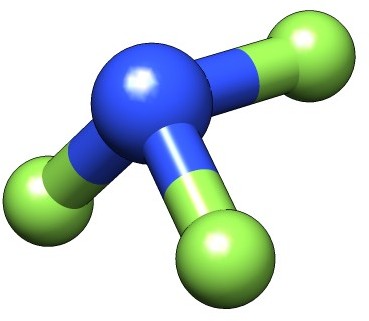
The molecular input file NF3.mol uses the experimental geometry and automatic symmetry detection.
INTGRL
NF3, exp.geom
daug-cc-pVQZ
C   2              A
        7.    1
N      0.000000000        0.0000000000        0.0000000000
LARGE BASIS aug-cc-pVDZ
        9.    3
F1     0.0000000000        .0000000000        1.3676000000
F2     1.3385030000       0.0000000000        -.2806030000
F3     -.3455290000       1.293136000         -.2806030000
LARGE BASIS aug-cc-pVDZ
FINISH
Generating the HF wave function
We first run a Hartree-Fock calculation to generate orbitals and corresponding energies using scf.inp
**DIRAC
.TITLE
NF3
.WAVE F
.ANALYZE
**INTEGRALS
*READIN
.UNCONT
**WAVE FUNCTIONS
.SCF
*SCF
.CLOSED SHELL
34
**ANALYZE
.MULPOP
*END OF
and the command:
pam --inp=scf --mol=NF3 --outcmo
You may notice in the output that DIRAC will center and rotate the molecule. It detects the full \(C_{3v}\) symmetry, but will run the calculation in the lower \(C_s\) symmetry, with reflection in the xy -plane, with the \(C_3\) rotation around the x -axis.
Magnetizabilities: first attempt
We first calculate the magnetizability using the input file cgo.inp
**DIRAC
.TITLE
NF3
.PROPERTIES
**GENERAL
.RKBIMP
**HAMILTONIAN
.URKBAL
**INTEGRALS
*READIN
.UNCONT
**WAVE FUNCTIONS
.SCF
*SCF
.CLOSED SHELL
34
**PROPERTIES
.MAGNET
*NMR
.USECM
*END OF
where the (common) gauge origin has been set to the center of mass using the .USECM keyword. Notice that we use .RKBIMP (? .RKBIMP ) to convert our molecular coefficients from restricted to unrestricted kinetic balance (RKB \(\rightarrow\) UKB), the former employed for the generation of orbitals, and the latter employed for the response calculations, indicated by .URKBAL. This corresponds to the use of simple magnetic balance. The calculation is run using:
pam --inp=cgo --mol=NF3 --incmo
and gives the total magnetizability tensor
                                 Bx                  By                  Bz


            Bx        -6.311410457817     -0.000000000000     -0.000004485788
            By        -0.000000000000     -6.311410738039     -0.000000000000
            Bz         0.000000339879     -0.000000000000     -6.753534842323
here reported in atomic units \(e^2a_0^2/m_e\), corresponding to 7.89104 \(\cdot 10^{-29}\) J/T.
Magnetizabilities using LAOs
We now activate LAOs using the input file lao.inp
**DIRAC
.TITLE
NF3
.PROPERTIES
**GENERAL
.RKBIMP
**HAMILTONIAN
.URKBAL
**INTEGRALS
*READIN
.UNCONT
**WAVE FUNCTIONS
.SCF
*SCF
.CLOSED SHELL
34
**PROPERTIES
.MAGNET
*NMR
.LONDON
*END OF
which gives the total magnetizability tensor
                                 Bx                  By                  Bz


            Bx        -5.215860172448      0.000000000000     -0.000000702830
            By         0.000000000000     -5.215856642085     -0.000000000000
            Bz         0.000002183587     -0.000000000000     -4.570158593223
which is markedly different from the CGO. The question now is: Which result is ‘best’ ? From microwave spectroscopy (see []) the magnetizability anisotropy, defined as
has been found to be -0.63 \((\pm 0.32)\ e^2a_0^2/m_e\). With CGO and LAOs we obtain +0.4421 and -0.6457 \(e^2a_0^2/m_e\), respectively, clearly favoring the LAO calculation. However, it very often happens that one gets the right answer for the wrong reason, so let us investigate the gauge-origin independence of the result as well as basis set convergence.
Gauge-origin dependence
To investigate gauge-origin dependence we do a CGO and LAO calculation with the gauge origin placed at:
**INTEGRALS
.GO ANG ! gauge origin in Angstrom
10.00 0.0 0.0
that is, along the \(C_3\) axis. Please note that when shifting the gauge origin in this manner you should limit the gauge origin to symmetry-independent points, that is, you should stay on symmetry elements like the xy mirror plane in this case. The CGO calculation now gives
                                 Bx                  By                  Bz

            Bx        -6.753534785034     -0.000019708625     -0.000000000000
            By         0.000016616881   -134.461048086921     -0.000000000000
            Bz        -0.000000000000     -0.000000000000   -134.460100713107
We see that the parallel component \(\zeta_\parallel\) is unchanged, whereas the perpendicular component \(\zeta_\perp\) is dramatically different. With LAOs we get
                                 Bx                  By                  Bz

            Bx        -4.570158198807     -0.000014273103     -0.000000000001
            By         0.000001955079     -5.215956665783      0.000000000000
            Bz        -0.000000000001      0.000000000000     -5.215972281121
where the numerical differences with respect to the original calculation is below the convergence threshold of the linear response calculation. We can therefore see that the use of LAOs removes the gauge dependence in the finite basis approximation.
Basis-set convergence
The basis set convergence is illustrated by the following table, taken from [Ilias2013], showing CGO(LAO) magnetizabilities (in \(e^2a_0^2/m_e\)) for a wide range of basis sets.
Basis |
\(\zeta_{\parallel}\) |
\(\zeta_{\perp}\) |
\(\zeta_{iso}\) |
\(\zeta_{ani}\) |
DZ |
-14.83 (-4.27) |
-9.78 (-4.87) |
-11.47 (-4.67) |
+5.04 (-0.60) |
TZ |
-7.88 (-4.36) |
-6.52 (-4.96) |
-6.97 (-4.76) |
+1.37 (-0.60) |
QZ |
-5.65 (-4.43) |
-5.54 (-5.04) |
-5.58 (-4.83) |
+0.11 (-0.61) |
aug-DZ |
-6.75 (-4.57) |
-6.31 (-5.22) |
-6.46 (-5.00) |
+0.44 (-0.65) |
aug-TZ |
-5.01 (-4.64) |
-5.42 (-5.24) |
-5.28 (-5.04) |
-0.41 (-0.60) |
aug-QZ |
-4.70 (-4.64) |
-5.26 (-5.24) |
-5.08 (-5.04) |
-0.56 (-0.60) |
d-aug-DZ |
-6.37 (-4.57) |
-6.18 (-5.22) |
-6.24 (-5.00) |
+0.19 (-0.65) |
d-aug-TZ |
-5.01 (-4.69) |
-5.45 (-5.27) |
-5.31 (-5.08) |
-0.44 (-0.58) |
d-aug-QZ |
-4.76 (-4.68) |
-5.31 (-5.28) |
-5.13 (-5.08) |
-0.55 (-0.60) |
The basis set convergence is seen to be dramatically different, again clearly in favour of LAOs.