A Hartree-Fock calculation with the polarizable embedding (PE) model
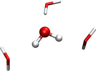
In this tutorial we will cover the set up of a Hartree-Fock calculation using the polarizable embedding (PE) model ([Olsen2010], [Olsen2011]) to include effects from a surrounding environment. Our example concerns a solvent effect, but the PE model is general and can also handle other environments (e.g. proteins or mixed solvents). The implementation of the model in DIRAC is documented in the paper [Hedegaard2017], and we refer to this paper for further technical details. Our target system for this tutorial is a water molecule surrounded (or “microsolvated”) by three other water molecules. The system is shown in the figure below. The molecule in ball-and-stick representation is the one that is described with Hartree-Fock, and the three other water molecules are represented by an explicit PE potential. The underlying structure is abstracted from an MD simulation on a larger water cluster [Kongsted2002]. In real production calculations, PE would be used for the full system (PE is intended for much larger environments than three molecules), but this system is sufficient to show how the setup works.
The current implementation employs the external library PElib for the PE-related tasks. The module is activated by the .PEQM keyword under the **HAMILTONIAN section. A few additional (but also very simple) examples can be found in the test directories.
The .mol file (h2o.mol) for the central water molecule is shown below:
INTGRL
H2O structure, taken from Kongsted et al. (2002)
------------------------
C   2    0
        8.0   1
O    0.0000000000   0.000000000    0.0000000000
LARGE BASIS 6-31++G
        1.0   2
H   -1.4301431032   0.000000000    1.1073930799
H    1.4301431032   0.000000000    1.1073930799
LARGE BASIS 6-31++G
FINISH
The more experienced user will notice that the format is exactly the same as for a vacuum calculation. The .inp file (pe-hf.inp) is given below:
**DIRAC
.TITLE
H2O with PE
.WAVE FUNCTION
**HAMILTONIAN
.PEQM            ! activate polarizable embedding
**INTEGRALS
*TWOINT
.SCREEN
1.0D-12
*READIN
.UNCONT
**WAVE FUNCTIONS
.SCF
*SCF
.CLOSED SHELL
10
*END OF
PElib is activated by the .PEQM keyword under **HAMILTONIAN. Specification of .PEQM will thus make the program calculate the PE-specific term of the Fock (or Kohn-Sham) matrix and add them to the vacuum part (see Eqs. (19)-(22) in [Hedegaard2017]). Additional PE-related keywords are given under the *PEQM section. This potential has to be generated but for now we can use the pre-generated potential (3_h2o.pot) given below
   ! potential: 3_h2o.pot
   ! ------------------
   ! Multipole moments:
   ! ------------------
   !        TYPE: DALTON-LoProp
   !      METHOD: DFT
   !      XC-FUN: CAMB3LYP
   !   BASIS SET: loprop-6-31+G*
   ! -----------------
   ! Polarizabilities:
   ! -----------------
   !        TYPE: DALTON-LoProp
   !      METHOD: DFT
   !      XC-FUN: CAMB3LYP
   !   BASIS SET: loprop-6-31+G*
   ! -----------------
   @COORDINATES
   9
   AA
   O     2.36500000   -0.26700000    1.17000000
   H     2.26100000   -1.10300000    1.62300000
   H     3.13200000   -0.39000000    0.61100000
   O     0.60500000   -1.46500000   -2.08000000
   H     1.56100000   -1.47200000   -2.03300000
   H     0.33300000   -0.92000000   -1.34100000
   O    -2.76000000   -0.37900000    1.04500000
   H    -3.11300000   -0.71800000    0.22300000
   H    -3.08300000   -0.98500000    1.71200000
   @MULTIPOLES
   ORDER 0
   9
    1   -0.71214000
    2    0.35613000
    3    0.35601000
    4   -0.71172000
    5    0.35592000
    6    0.35580000
    7   -0.71195000
    8    0.35605000
    9    0.35589000
   ORDER 1
   9
    1    0.18080000   -0.26163000   -0.02886000
    2    0.02828000    0.15363000   -0.09058000
    3   -0.14340000    0.01302000    0.10892000
    4    0.18641000    0.14653000    0.21409000
    5   -0.18048000    0.00772000   -0.00000000
    6    0.06166000   -0.10108000   -0.13640000
    7   -0.18419000   -0.25746000   -0.04234000
    8    0.06167000    0.05571000    0.16046000
    9    0.05571000    0.10834000   -0.13341000
   ORDER 2
   9
    1   -4.26483000    0.09135000   -0.61915000   -4.18829000   -0.42704000   -4.30439000
    2   -0.44339000    0.02690000   -0.02255000   -0.13348000   -0.16450000   -0.36591000
    3   -0.19077000   -0.05251000   -0.18965000   -0.43313000    0.03146000   -0.31920000
    4   -3.75473000   -0.26370000   -0.29217000   -4.64173000    0.46544000   -4.36137000
    5   -0.04700000    0.00328000    0.02886000   -0.45150000    0.00785000   -0.44444000
    6   -0.41521000   -0.05871000   -0.07885000   -0.32164000    0.18442000   -0.20640000
    7   -4.75797000    0.31610000    0.08263000   -4.49207000   -0.18934000   -3.50706000
    8   -0.39388000    0.06405000    0.12905000   -0.39012000    0.12442000   -0.15864000
    9   -0.40305000    0.09738000   -0.09242000   -0.27989000   -0.17467000   -0.26011000
   @POLARIZABILITIES
   ORDER 1 1
   9
    1    4.27640000    0.35715000    0.52792000    3.89073000    0.26437000    4.59489000
    2    0.42029000    0.22994000    0.06545000    2.24667000   -0.89940000    0.97487000
    3    1.98744000   -0.26213000   -0.97060000    0.39136000    0.31466000    1.26588000
    4    3.86307000   -0.04205000   -0.13378000    4.67372000   -0.64393000    4.23650000
    5    2.71461000    0.04981000    0.19272000    0.51208000   -0.15905000    0.42003000
    6    0.43352000   -0.33472000   -0.47532000    1.31851000    0.93618000    1.89744000
    7    4.64952000   -0.67410000   -0.13594000    4.15079000    0.04738000    3.96576000
    8    0.88018000    0.20475000    0.75848000    0.75651000    0.80933000    2.00627000
    9    0.82484000    0.41178000   -0.61423000    1.44166000   -1.04482000    1.38018000
   EXCLISTS
   9 3
    1 2 3
    2 1 3
    3 1 2
    4 5 6
    5 4 6
    6 4 5
    7 8 9
    8 7 9
    9 7 8
The potential contains coordinates for three water molecules surrounding the central water. The three water molecules are represented by multipoles up to 2nd order (charges, dipole, and quadrupoles) and anisotropic dipole-dipole polarizabilities. Now we have all the ingredients needed to start the calculation:
pam --inp=pe-hf.inp --mol=h2o.mol --pot=3_h2o.pot
The output file will be named pe-hf_h2o_3_h2o.out. When the calculation is converged, the final energy report contains an additional entry; the “Embedding energy”, which is also included in the total energy:
                                TOTAL ENERGY
                                ------------

Electronic energy                        :    -85.261494639123399

Other contributions to the total energy
Nuclear repulsion energy                 :      9.195432882420004
Embedding energy                         :     -0.063104845058299
SS Coulombic correction                  :      0.000000028807992

Sum of all contributions to the energy
Total energy                             :    -76.108136383446379
A PE-DFT calculation can be run in exactly the same manner, but by additionally specifying DFT under the **HAMILTONIAN section (see e.g. the follow-up tutorial).
Things to note
- Currently, the PE model is only implemented for Hartree-Fock and Kohn-Sham DFT.
- X2C Hamiltonian works with the PE model, but the embedding operator is not transformed.