A TDDFT study of carbon monoxide
Introduction
To illustrate the TDDFT capabilities of DIRAC we will consider excited states of the carbon monoxide molecule. The experimental spectrum can be found here . Note that this source gives only adiabatic excitation energies \(T_e\), that is, the energy difference between the minima of the potential curve of the ground and excited state, whereas the TDDFT calculations give vertical excitation energies \(T_v\). The experimental adiabatic excitation energies has been converted to vertical ones by [Nielsen_JCP1980]. We will begin this tutorial in spinfree mode to faciliate the connection to the non-relativistic domain. In the following we employ the molecular input file CO.mol
INTGRL
Carbon monoxide
Dunning aug-cc-pVDZ
C   2              A
        6.    1
C        0.0000000000000     0.0000000000000     0.0000000000000
LARGE BASIS aug-cc-pVDZ
        8.    1
O        0.0000000000000     0.0000000000000     1.128323
LARGE BASIS aug-cc-pVDZ
FINISH
Here we do not provide any symmetry information, meaning that we ask DIRAC to detect it. DIRAC will find that the full group is \(C_{\infty v}\). With spin-orbit coupling DIRAC will then activate linear supersymmetry, but in the spin-orbit free case it will simply use the highest Abelian single point group, that is \(C_{2v}\). Irreps of \(C_{\infty v}\) and \(C_{2v}\) correlate as follows:
| \(C_{\infty v}\) | \(C_{2v}\) |
|---|---|
| \(\Sigma^{+}\) | \(A_1\) |
| \(\Sigma^{-}\) | \(A_2\) |
| \(\Pi\) | \(B_1, B_2\) |
| \(\Delta\) | \(A_1, A_2\) |
Ground state electronic structure
Before actually doing TDDFT let us first have a look at the electronic structure of the ground state of CO. We therefore carry out Kohn-Sham DFT using the PBE functional and the eXact 2-Component (X2C) Hamiltonian followed by Mulliken population analysis using the input file SCF.inp
**DIRAC
.TITLE
CO
.WAVE FUNCTIONS
.ANALYZE
**HAMILTONIAN
.SPINFREE
.X2C
.DFTAUTO    ! uses xcfun
PBE
**INTEGRALS
*TWOINT
.SCREEN
1.0D-12
*READIN
.UNCONT
**WAVE FUNCTIONS
.SCF
*SCF
.CLOSED SHELL
14
**ANALYZE
.MULPOP
*MULPOP
.VECPOP
1..10
*END OF
Based on orbital energies and the Mulliken population analysis we can set up the following MO diagram:
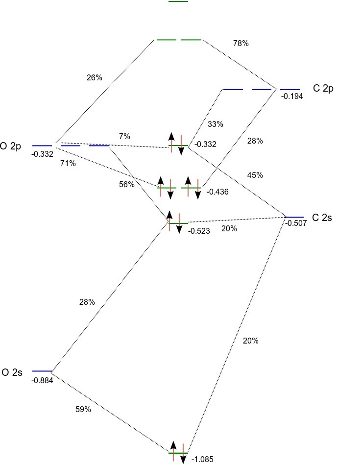
(Orbital energies for the atoms were obtained from atomic calculations using fractional occupation)
According to the above MO diagram the valence electron configuration of carbon monoxide is \(1\sigma^{2}2\sigma^{2}1\pi^{4}3\sigma^{2}\). From projection analysis we find that the electron configurations of the carbon and oxygen atoms in the molecule are \(1s^{2.0}2s^{2.0}2p^{2.0}\) and \(1s^{2.0}2s^{1.7}2p^{4.3}\) , respectively, with a slight negative charge of -0.3 on oxygen. We note that the HOMO is a \(\sigma\) orbital dominated (~90 %) by carbon (2s,2p), whereas the doubly degenerate LUMO is a \(\pi\) orbital with about 75% C 2p and 25% O 2p. The LUMO+1 is \(\sigma\) orbital with a combination of carbon and oxygen 3s dominated by the former atom.
Excited states
Preparing the input files
The excited states will be calculated in a “bottoms-up” fashion for each irrep by expansion of the solution vector in trial vector [Bast2009]. For each irrep the user specifies the number of desired excitations. It may be a good idea of including some extra excitations in case of root flipping during the iterative solution of the TDDFT equations. We are working within the adiabatic approximation of TDDFT and consider single excitations from a closed-shell ground state. The final states will be therefore be singlet or triplets in the spin-orbit free case. We need to tell DIRAC how these states are distributed on the four irreps of \(C_{2v}\). At this point we should emphasize that DIRAC will employ the total symmetry of the final states, that is the combined spin and spatial symmetry. A singlet spin function is totally symmetric (\(A_1\)), whereas the triplet spin functions transform as rotations. We know the triplet functions as:
but for our purposes it will be more convenient to form the combinations:
which transform as rotations \(R_x\left(B_{2}\right)\) , \(R_y\left(B_{1}\right)\) and \(R_z\left(A_{2}\right)\) , respectively. For a given point group you find the symmetry of the rotations in most standard character tables (for instance here ).
As an example of how to determine total symmetry of the final states let us consider single excitations HOMO into the LUMO (\(\pi\)) and LUMO+1 (\(\sigma\)) orbitals. This leads to \(2 \times\ 6 = 12\) determinants which translate into the following final states:
| Configuration | States |
|---|---|
| \(3\sigma^{-1}2\pi^{1}\) | \(^{1,3}\Pi\) |
| \(3\sigma^{-1}4\sigma^{1}\) | \(^{1,3}\Sigma\) |
We can now set up the following correlation of states:
| State | Spin | Spatial | Spin \(\otimes\) Spatial |
|---|---|---|---|
| \(^1\Sigma\) | \(A_1\) | \(A_1\) | \(A_1\) |
| \(^1\Pi_{x,y}\) | \(A_1\) | \(B_{1}, B_{2}\) | \(B_{1}, B_{2}\) |
| \(^3\Sigma\) | \(B_{2}, B_{1}, A_{2}\) | \(A_1\) | \(B_{2}, B_{1}, A_{2}\) |
| \(^3\Pi_{x,y}\) | \(B_{2}, B_{1}, A_{2}\) | \(B_{1}, B_{2}\) | \(\left(A_2, A_{1}, B_2\right), \left(A_1, A_2, B_2\right)\) |
(The group multiplication table is found in the DIRAC output.)
Counting total symmetries we find that the 12 microstates are evenly distributed amongst the four irreps of \(C_{2v}\):
| Irrep | Valence-excited state | |
|---|---|---|
| 1 | \(A_1\) | \(^1\Sigma, ^{3(y)}\Pi_{x}, ^{3(x)}\Pi_{y}\) |
| 2 | \(B_1\) | \(^{1}\Pi_{x}, ^{3(y)}\Sigma, ^{3(z)}\Pi_{y}\) |
| 3 | \(B_2\) | \(^{1}\Pi_{y}, ^{3(x)}\Sigma, ^{3(z)}\Pi_{x}\) |
| 4 | \(A_2\) | \(^{3(z)}\Sigma, ^{3(x)}\Pi_{x}, ^{3(y)}\Pi_{y}\) |
Note that the order of the irreps follows the output of DIRAC.
We now set up the following menu file TDDFT.inp for our calculation
**DIRAC
.TITLE
CO
.WAVE FUNCTIONS
.ANALYZE
.PROPERTIES
**HAMILTONIAN
#.SPINFREE
.X2C
.DFT
CAMB3LYP
**INTEGRALS
*READIN
.UNCONT
**WAVE FUNCTIONS
.SCF
*SCF
.CLOSED SHELL
14
**ANALYZE
.MULPOP
*MULPOP
.VECPOP
1..10
**PROPERTIES
*EXCITATION
#A1 :
.EXCITA
1 10
#B1 :
.EXCITA
2 10
#B2 :
.EXCITA
3 10
#A2 :
.EXCITA
4 10
.ANALYZE
.INTENS
0
*END OF
We base our TDDFT calculation on the long-range corrected CAMB3LYP functional [Yanai_CPL2004] which provides a better description of Rydberg and charge-transfer excitations than standard continuum functionals. We furthermore ask for oscillator strengths within the electric dipole approximation. Finally we ask for analysis of what orbitals contribute to the various excitations. For this the Mulliken population analysis may come in handy as reference.
Looking at the output
Energy levels
After running the calculation, let us now look at the output. There is output for each symmetry, but we go directly to the final output at the end where we first find a list of levels
 Level   Rel eigenvalue     Abs eigenvalue      Total Energy    Degeneracy

    0     0.0000000000      0.000000000000     -113.360751211913 (   1 * )
    1     0.2179684416      0.217968441552     -113.142782770361 (   6 * )
    2     0.2920913720      0.292091372039     -113.068659839874 (   3 * )
    3     0.3118502990      0.311850298956     -113.048900912957 (   2 * )
    4     0.3196082474      0.319608247388     -113.041142964524 (   3 * )
    5     0.3196082747      0.319608274709     -113.041142937203 (   3 * )
    6     0.3571903408      0.357190340783     -113.003560871130 (   4 * )
    7     0.3713721017      0.371372101748     -112.989379110165 (   1 * )
    8     0.3713721244      0.371372124437     -112.989379087475 (   1 * )
    9     0.3772336576      0.377233657576     -112.983517554337 (   3 * )
   10     0.4005688143      0.400568814285     -112.960182397628 (   1 * )
   11     0.4055211488      0.405521148807     -112.955230063105 (   3 * )
   12     0.4148565572      0.414856557192     -112.945894654721 (   1 * )
   13     0.4154753076      0.415475307619     -112.945275904294 (   6 * )
   14     0.4211386601      0.421138660103     -112.939612551809 (   2 * )
   15     0.4421501229      0.442150122889     -112.918601089024 (   1 * )
The degeneracies indicated in parenthesis for each level generally arise from both spatial and spin degrees of freedom. DIRAC assumes degeneracy when energies are within \(1.0\cdot10^{-9}\ E_h\). As we shall see this is not a foolproof scheme.
To learn more about the nature of the excitated states we look at the following list of energy levels, now in other units (eV and cm \(^{-1}\)) and with symmetry information:
 Symmetry Classification in the Abelian subgroup

 Level  eigenvalue (eV)  Eigenvalue (cm-1)  1A1 |1B1 |1B2 |1A2 |3A1 |3B1 |3B2 |3A2 |

    0        0.000000000          0.000000     1|   0|   0|   0|   0|   0|   0|   0|
    1        5.931222840      47838.543340     0|   0|   0|   0|   0|   3|   3|   0|
    2        7.948210323      64106.646178     0|   0|   0|   0|   3|   0|   0|   0|
    3        8.485878060      68443.229378     0|   1|   1|   0|   0|   0|   0|   0|
    4        8.696982570      70145.902250     0|   0|   0|   0|   0|   0|   0|   3|
    5        8.696983313      70145.908246     0|   0|   0|   0|   3|   0|   0|   0|
    6        9.719643323      78394.218340     0|   0|   0|   1|   0|   0|   0|   3|
    7       10.105548659      81506.755099     0|   0|   0|   1|   0|   0|   0|   0|
    8       10.105549276      81506.760079     1|   0|   0|   0|   0|   0|   0|   0|
    9       10.265049702      82793.217903     0|   0|   0|   0|   3|   0|   0|   0|
   10       10.900031599      87914.692818     1|   0|   0|   0|   0|   0|   0|   0|
   11       11.034791472      89001.604611     0|   0|   0|   0|   3|   0|   0|   0|
   12       11.288820849      91050.489924     1|   0|   0|   0|   0|   0|   0|   0|
   13       11.305657905      91186.289946     0|   0|   0|   0|   0|   3|   3|   0|
   14       11.459765561      92429.252144     0|   1|   1|   0|   0|   0|   0|   0|
   15       12.031516531      97040.735192     0|   0|   0|   0|   0|   1|   0|   0|
The first level is simply the ground state. The reference state for calculation excitation energies is presently limited to closed-shell and so this is \(^1A_1\) (\(C_{2v}\)), corresponding to \(^1\Sigma^+\) of \(C_{v\infty}\). Linear (super)symmetry is not implemented for spin-orbit free calculations, so DIRAC gives symmetry information with respect to \(C_{2v}\). DIRAC, however, is able to separate spin and spatial symmetries. We see for instance the the next level is six-fold degenerate with equal contributions from \(^3B_1\) and \(^3B_2\). Looking at the above correspondence table between \(C_{2v}\) and \(C_{v\infty}\) that a degenerate level of \(B_1\) and \(B_2\) spatial symmetries corresponds to a \(\Delta\) term, so we identify the first excited level of CO as \(^3\Delta\). The correspondence table also allows us to distinguish mirror symmetry about the molecular axis for \(\Sigma\) states, so we identify the second excited state as \(^{3}\Sigma^{+}\). Proceeding in this manner, we also see some failures of the degeneracy detection in DIRAC. Level 4 and 5 are classified as \(^3A_1\) and \(^3A_2\), respectively, and are clearly components of a \(^3\Delta\) state. Reducing the threshold for degeneracies would bring them together, as well as level 7 (\(^1A_2\)) and 8 (\(^1A_1\)), which are component of a \(^1\Delta\) state. However, level 6 is seen to contain both a singlet \(^1A_2\) (\(^1\Sigma^-\)) and a triplet \(^3A_2\) (\(^3\Sigma^-\)) which are clearly not allowed to mix without spin-orbit interaction, so here a larger threshold would be needed to distinguish them.
Below we give a summary of results obtained with a variety of functionals available in DIRAC. The assignment and energy of states may be compared to [Tozer_JCP1998].
| \(T_e\) | \(T_v\) | CAMB3LYP | LDA | PBE | PBE0 | BLYP | B3LYP | |
|---|---|---|---|---|---|---|---|---|
| \(a\ ^{3}\Pi\) | 6.04 | 6.32 | 5.93 | 5.98 | 5.77 | 5.76 | 5.85 | 5.88 |
| \(a\ ^{3}\Sigma^{+}\) | 6.92 | 8.51 | 7.95 | 8.43 | 8.12 | 7.85 | 8.10 | 7.93 |
| \(A\ ^{1}\Pi\) | 8.07 | 8.51 | 8.49 | 8.19 | 8.26 | 8.45 | 8.25 | 8.41 |
| \(d\ ^{3}\Delta\) | 7.58 | 9.36 | 8.70 | 9.21 | 8.78 | 8.64 | 8.72 | 8.66 |
| \(e\ ^{3}\Sigma^{-}\) | 7.96 | 9.88 | 9.72 | 9.89 | 9.87 | 9.79 | 9.79 | 9.73 |
| \(I\ ^{1}\Sigma^{-}\) | 8.07 | 9.88 | 9.72 | 9.89 | 9.87 | 9.79 | 9.79 | 9.73 |
| \(D\ ^{1}\Delta\) | 8.17 | 10.23 | 10.11 | 10.36 | 10.21 | 10.21 | 10.03 | 10.05 |
| \(b\ ^{3}\Sigma^{+}\) | 10.39 | 10.4 | 10.27 | 9.59 | 9.35 | 10.12 | 9.29 | 9.95 |
| \(B\ ^{1}\Sigma^{+}\) | 10.78 | 10.78 | 10.90 | 9.95 | 9.78 | 10.72 | 9.65 | 10.43 |
| \(j\ ^{3}\Sigma^{+}\) | 11.28 | 11.3 | 10.27 | 10.37 | 10.09 | 10.84 | 10.09 | 10.71 |
| \(C\ ^{1}\Sigma^{+}\) | 11.40 | 11.4 | 11.29 | 10.68 | 10.56 | 11.25 | 10.49 | 11.05 |
| \(E\ ^{1}\Pi\) | 11.52 | 11.53 | 11.46 | 10.70 | 10.58 | 11.36 | 10.49 | 11.13 |
| \(c\ ^{3}\Pi\) | 11.55 | 11.55 | 11.31 | 10.31 | 10.31 | 11.12 | 10.30 | 10.97 |
| MAE (all states) | 0.29 | 0.49 | 0.62 | 0.29 | 0.68 | 0.39 | ||
| MAE (valence) | 0.30 | 0.15 | 0.26 | 0.31 | 0.31 | 0.33 | ||
| MAE (Rydberg) | 0.29 | 0.89 | 1.05 | 0.26 | 1.11 | 0.46 |
For all functionals we provide the mean absolute error (MAE), and it can indeed be seen that the performance of CAMB3LYP is quite good. PBE0 is also display nice performance, whereas its GGA equivalent comes out significantly worse. However, if we do separate error analysis of the valence states (the first seven states) and the Rydberg states (the last six states), we see that PBE performs well for the valence states, but not for the Rydberg states. This is connected to the wrong asymptotic behaviour of LDA/GGA functionals.
The performance of standard LDA/GGA functionals can be improved by invoking asymptotic corrections. One option is the statistical average of orbital potentials (SAOP). Below we show the result of SAOP-corrected functionals.
| SAOP-corrected | \(T_e\) | \(T_v\) | SAOP | LDA | PBE | PBE0 | BLYP | B3LYP |
|---|---|---|---|---|---|---|---|---|
| \(a\ ^{3}\Pi\) | 6.04 | 6.32 | 6.33 | 6.11 | 5.76 | 5.76 | 5.84 | 5.87 |
| \(a\ ^{3}\Sigma^{+}\) | 6.92 | 8.51 | 8.65 | 8.47 | 7.88 | 7.88 | 8.19 | 8.00 |
| \(A\ ^{1}\Pi\) | 8.07 | 8.51 | 8.60 | 8.47 | 8.57 | 8.57 | 8.61 | 8.64 |
| \(d\ ^{3}\Delta\) | 7.58 | 9.36 | 9.39 | 9.30 | 8.64 | 8.64 | 8.79 | 8.71 |
| \(e\ ^{3}\Sigma^{-}\) | 7.96 | 9.88 | 10.04 | 10.00 | 9.77 | 9.77 | 9.84 | 9.76 |
| \(I\ ^{1}\Sigma^{-}\) | 8.07 | 9.88 | 10.04 | 10.00 | 9.77 | 9.77 | 9.84 | 9.76 |
| \(D\ ^{1}\Delta\) | 8.17 | 10.23 | 10.50 | 10.49 | 10.27 | 10.27 | 10.39 | 10.31 |
| \(b\ ^{3}\Sigma^{+}\) | 10.39 | 10.4 | 10.48 | 10.87 | 10.49 | 10.49 | 10.21 | 10.52 |
| \(B\ ^{1}\Sigma^{+}\) | 10.78 | 10.78 | 10.97 | 11.25 | 11.21 | 11.21 | 10.83 | 11.22 |
| \(j\ ^{3}\Sigma^{+}\) | 11.28 | 11.3 | 11.42 | 11.70 | 11.34 | 11.34 | 11.20 | 11.43 |
| \(C\ ^{1}\Sigma^{+}\) | 11.40 | 11.4 | 11.73 | 11.97 | 11.80 | 11.80 | ||
| \(E\ ^{1}\Pi\) | 11.52 | 11.53 | 11.89 | 11.97 | 11.97 | |||
| \(c\ ^{3}\Pi\) | 11.55 | 11.55 | 11.76 | 11.73 | 11.68 | 11.68 | 11.42 | 11.70 |
| MAE (all states) | 0.17 | 0.24 | 0.29 | 0.29 | 0.20 | 0.26 | ||
| MAE (valence) | 0.12 | 0.12 | 0.32 | 0.32 | 0.24 | 0.29 | ||
| MAE (Rydberg) | 0.21 | 0.42 | 0.25 | 0.25 | 0.12 | 0.21 |
Orbital contributions
We can also get information about dominant (single) excitations leading to each excited state. We then go to the section starting with:
Analysis of response solution vectors
-------------------------------------
For the first excitation of \(A_1\) total (space+spin) symmetry we find for example
** E solution vectors : PP EXCITATIONA1  Irrep: A1  Trev:   1 Length:        441
 Freq.:   0.217968 Norm:   0.71160560E+00 Residual norm:   0.29E-05
   Dominant inactive orbitals:
     7(E1 ) 99.56%
   Dominant virtual orbitals:
     8(E1 ) 87.92%
    12(E1 ) 10.80%
   Excitation amplitudes larger than threshold   0.34E-01

        7(i:E1 ) --->      8(v:E1 )  0.66634917E+00
        7(i:E1 ) --->     12(v:E1 )  0.23316913E+00
        7(i:E1 ) --->     15(v:E1 )  0.55294831E-01
        7(i:E1 ) --->     24(v:E1 )  0.41863343E-01
        4(i:E1 ) --->      8(v:E1 )  0.34734025E-01
This is an excitation to the first \(^3\Delta\) state, combining a \(T_y\) spin function with \(B_1\) spatial symmetry. The dominant inactive orbital is orbital 7 and if we look at the Mulliken population analysis we find
* Electronic eigenvalue no.  7: -0.4549728114484       (Occupation : f = 1.0000)  sym= A1
==========================================================================================

* Gross populations greater than 0.00010

Gross     Total   |    L A1 C  s      L A1 C  pz     L A1 C  dxx    L A1 C  dyy    L A1 C  dzz    L A1 O  s      L A1 O  pz
--------------------------------------------------------------------------------------------------------------------------------
 alpha    1.0000  |      0.5192         0.3567         0.0081         0.0081        -0.0122         0.0290         0.0872
 beta     0.0000  |      0.0000         0.0000         0.0000         0.0000         0.0000         0.0000         0.0000
showing that this is the HOMO, which is a \(\sigma\) orbital with 51 % carbon s and 36 % carbon p character. The dominant virtual orbital is orbital 8
* Electronic eigenvalue no.  8:  0.116603897E-01       (Occupation : f = 0.0000)  sym= B1
==========================================================================================

* Gross populations greater than 0.00010

Gross     Total   |    L B1 C  px     L B1 C  dxz    L B1 O  px     L B1 O  dxz
-----------------------------------------------------------------------------------
 alpha    0.0000  |      0.0000         0.0000         0.0000         0.0000
 beta     1.0000  |      0.9302         0.0039         0.0622         0.0037
which is clearly a \(\pi\) orbital dominated by carbon \(p_x\).
Oscillator strenghts
DIRAC also allows provides oscillator strenghts corresponding to the calculated (single) excitations. The general definition of an oscillator strenght is
where \(\hbar\omega_{0n}\) and \(T_{0n}\) are the corresponding excitation energy and transition moment, respectively. The calculation of oscillator strengths is invoked through:
.INTENS
0
which means that we ask for oscillator strengths to order zero in the wave vector. So far only the zeroth-order, corresponding to the electric dipole approximation, has been implemented in DIRAC. The isotropic dipole length-dipole length oscillator strenghts are given as
and are found to be
* ISOTROPIC DL-DL OSCILLATOR STRENGTHS (f)
==========================================
DL = dipole length
Rate = Dipole radiation rate (s-1)
Lifetime = corresponding radiation lifetime (s)

Level     Frequency     f             Rate           Lifetime
------------------------------------------------------------------------
   11     0.3118502990  0.08693603    0.27165E+09    0.36813E-08   1B1
   12     0.3118502990  0.08693603    0.27165E+09    0.36813E-08   1B2
   28     0.4005688143  0.00272236    0.14035E+08    0.71251E-07   1A1
   32     0.4148565572  0.20007880    0.11064E+10    0.90384E-09   1A1
   39     0.4211386601  0.05287740    0.30132E+09    0.33187E-08   1B1
   40     0.4211386601  0.05287740    0.30132E+09    0.33187E-08   1B2
------------------------------------------------------------------------
Sum of oscillator strenghts:      0.48243
DIRAC will also list the corresponding rate of spontaneous emission
and lifetime. This is a spin-orbit free calculation and so we only see oscillator strength to singlet states (clearly dominated by \(C\ ^{1}\Sigma^{+}\)). Things change is we activate spin-orbit interaction (that is, remove the .SPINFREE keyword). We see that the energy levels split up
 Level   Rel eigenvalue     Abs eigenvalue      Total Energy    Degeneracy

    0     0.0000000000      0.000000000000     -113.360753485853 (   1 * )
    1     0.2177547093      0.217754709334     -113.142998776518 (   1 * )
    2     0.2177548380      0.217754838019     -113.142998647834 (   1 * )
    3     0.2179681805      0.217968180514     -113.142785305339 (   2 * )
    4     0.2181824353      0.218182435267     -113.142571050585 (   2 * )
    5     0.2920874527      0.292087452684     -113.068666033168 (   2 * )
    6     0.2920912009      0.292091200866     -113.068662284987 (   1 * )
    7     0.3118487146      0.311848714618     -113.048904771234 (   2 * )
    8     0.3194494002      0.319449400172     -113.041304085680 (   2 * )
    9     0.3196035504      0.319603550360     -113.041149935492 (   1 * )
   10     0.3196035730      0.319603573038     -113.041149912815 (   1 * )
   11     0.3197697432      0.319769743172     -113.040983742681 (   2 * )
   12     0.3571899385      0.357189938455     -113.003563547398 (   1 * )
   13     0.3571902595      0.357190259490     -113.003563226363 (   1 * )
   14     0.3571939385      0.357193938480     -113.003559547373 (   2 * )
   15     0.3713761730      0.371376172999     -112.989377312854 (   1 * )
   16     0.3713761911      0.371376191084     -112.989377294769 (   1 * )
   17     0.3772335792      0.377233579233     -112.983519906620 (   1 * )
   18     0.3772335957      0.377233595676     -112.983519890176 (   2 * )
   19     0.4005686574      0.400568657389     -112.960184828463 (   1 * )
   20     0.4055210631      0.405521063106     -112.955232422747 (   1 * )
   21     0.4055210675      0.405521067505     -112.955232418348 (   2 * )
   22     0.4148563890      0.414856389046     -112.945897096806 (   1 * )
   23     0.4154637988      0.415463798784     -112.945289687068 (   1 * )
   24     0.4154638709      0.415463870911     -112.945289614941 (   1 * )
   25     0.4154752275      0.415475227465     -112.945278258388 (   2 * )
   26     0.4154867238      0.415486723755     -112.945266762098 (   2 * )
   27     0.4211386128      0.421138612766     -112.939614873087 (   2 * )
   28     0.4420085600      0.442008560004     -112.918744925849 (   1 * )


 Total average:      -113.0232469850


 Relative real eigenvalues in other units;
 Symmetry Classification in the Abelian subgroup

 Level  eigenvalue (eV)  Eigenvalue (cm-1)   0+ | 0- | 1  | 2  | 3  |
    0        0.000000000          0.000000     1|   0|   0|   0|   0|
    1        5.925406891      47791.634541     0|   1|   0|   0|   0|
    2        5.925410393      47791.662784     1|   0|   0|   0|   0|
    3        5.931215737      47838.486049     0|   0|   2|   0|   0|
    4        5.937045905      47885.509532     0|   0|   0|   2|   0|
    5        7.948103672      64105.785980     0|   0|   2|   0|   0|
    6        7.948205666      64106.608610     0|   1|   0|   0|   0|
    7        8.485834948      68442.881656     0|   0|   2|   0|   0|
    8        8.692660117      70111.039316     0|   0|   0|   0|   2|
    9        8.696854757      70144.871371     0|   0|   0|   1|   0|
   10        8.696855374      70144.876348     0|   0|   0|   1|   0|
   11        8.701377093      70181.346477     0|   0|   2|   0|   0|
   12        9.719632375      78394.130040     1|   0|   0|   0|   0|
   13        9.719641111      78394.200499     0|   1|   0|   0|   0|
   14        9.719741222      78395.007943     0|   0|   2|   0|   0|
   15       10.105659443      81507.648635     0|   0|   0|   1|   0|
   16       10.105659935      81507.652605     0|   0|   0|   1|   0|
   17       10.265047570      82793.200709     0|   1|   0|   0|   0|
   18       10.265048018      82793.204318     0|   0|   2|   0|   0|
   19       10.900027329      87914.658383     1|   0|   0|   0|   0|
   20       11.034789140      89001.585802     0|   1|   0|   0|   0|
   21       11.034789260      89001.586767     0|   0|   2|   0|   0|
   22       11.288816274      91050.453020     1|   0|   0|   0|   0|
   23       11.305344733      91183.764049     0|   1|   0|   0|   0|
   24       11.305346696      91183.779879     1|   0|   0|   0|   0|
   25       11.305655723      91186.272354     0|   0|   2|   0|   0|
   26       11.305968553      91188.795498     0|   0|   0|   2|   0|
   27       11.459764272      92429.241755     0|   0|   2|   0|   0|
   28       12.027664409      97009.665730     1|   0|   0|   0|   0|
and that oscillator strength goes to more states
* ISOTROPIC DL-DL OSCILLATOR STRENGTHS (f)
==========================================
DL = dipole length
Rate = Dipole radiation rate (s-1)
Lifetime = corresponding radiation lifetime (s)

Level     Frequency     f             Rate           Lifetime
------------------------------------------------------------------------
    4     0.2179681805  0.00000024    0.37024E+03    0.27009E-02    1
    5     0.2179681805  0.00000024    0.37024E+03    0.27009E-02    1
    8     0.2920874527  0.00000161    0.44185E+04    0.22632E-03    1
    9     0.2920874527  0.00000161    0.44185E+04    0.22632E-03    1
   11     0.3118487146  0.08690291    0.27154E+09    0.36827E-08    1
   12     0.3118487146  0.08690291    0.27154E+09    0.36827E-08    1
   17     0.3197697432  0.00003112    0.10226E+06    0.97795E-05    1
   18     0.3197697432  0.00003112    0.10226E+06    0.97795E-05    1
   19     0.3571899385  0.00000082    0.33777E+04    0.29606E-03    0+
   21     0.3571939385  0.00000127    0.52073E+04    0.19204E-03    1
   22     0.3571939385  0.00000127    0.52073E+04    0.19204E-03    1
   26     0.3772335957  0.00000002    0.89752E+02    0.11142E-01    1
   27     0.3772335957  0.00000002    0.89752E+02    0.11142E-01    1
   28     0.4005686574  0.00272252    0.14036E+08    0.71246E-07    0+
   30     0.4055210675  0.00000011    0.59475E+03    0.16814E-02    1
   31     0.4055210675  0.00000011    0.59475E+03    0.16814E-02    1
   32     0.4148563890  0.20003957    0.11062E+10    0.90402E-09    0+
   34     0.4154638709  0.00004017    0.22276E+06    0.44892E-05    0+
   35     0.4154752275  0.00000033    0.18421E+04    0.54287E-03    1
   36     0.4154752275  0.00000033    0.18421E+04    0.54287E-03    1
   39     0.4211386128  0.05287687    0.30132E+09    0.33187E-08    1
   40     0.4211386128  0.05287687    0.30132E+09    0.33187E-08    1
   41     0.4420085600  0.00000421    0.26438E+05    0.37824E-04    0+
------------------------------------------------------------------------
Sum of oscillator strenghts:      0.48244
reflecting that triplet states “steal” intensity from singlet ones.