Hartree-Fock and DFT calculations in solution with the polarizable continuum model
This tutorial will cover the set up of an Hartree-Fock and a DFT calculation using the polarizable continuum model (PCM) to include solvent effects. The implementation of the PCM-SCF algorithm in DIRAC is documented in the recent paper [DiRemigio2015], to which the reader is referred for further technical details. The current implementation makes use of an external module for the PCM-related tasks. The module needs some input information to run properly.
As explained in the *PCMSOL section of the reference manual, a PCM calculation can be set up in two ways:
using three input files. The additional input file contains directives for the PCMSolver module;
using two input files. The additional directives in the inp file are forwarded to the PCMSolver module.
The second method is not as flexible as the first one and we will cover both in this tutorial.
For further details, please refer to the PCM documentation in the reference manual. Notice that the fact that a working implementation of the PCM-SCF algorithm gives access to geometry optimizations based on a numerical gradient and finite-field approaches to the calculation of response properties. The input files for DIRAC in these two cases need only be modified to include the directives relevant for the PCM calculation.
We will use the extremely simple examples contained in the test/pcm_energy directory. They are more than enough to show a simple workflow, possible gotchas and what to look for in a PCM output.
Warning
Calculations with the polarizable continuum model cannot exploit molecular point group symmetry and/or 2-component Hamiltonians.
The .mol file is prepared in the exact same manner as for an in vacuo calculation. In all the cases examined in the following, we will use the methane molecule with a STO-3G basis set:
INTGRL
methane (a standard MOLFDIR test at that geometry)
nonrelativistic contracted STO-3G basis
C   2    0
        6.    1
C   0.0000    0.0000    0.0000
LARGE BASIS STO-3G
        1.    4
H     .629889144   .629889144  .629889144
H    -.629889144  -.629889144  .629889144
H     .629889144  -.629889144 -.629889144
H    -.629889144   .629889144 -.629889144
LARGE BASIS STO-3G
FINISH
An Hartree-Fock calculation using three input files
In this example, the first input method will be used. We have to prepare three input files. The .inp file will feature some additional keywords:
**DIRAC
.WAVE FUNCTION
**HAMILTONIAN
.LEVY-LEBLOND
.PCM
*PCM
.SEPARATE
.PRINT
 6
**WAVE FUNCTION
.SCF
*SCF
.PRINT
1
*END OF
The .PCM keyword enables the addition of solvent terms to the Fock matrix. Details can be controlled through directives under the *PCM section (to which the reader is referred for further details) Using this input file a calculation using the Levy-Leblond Hamiltonian with PCM will be performed. Notice that the nuclear and electronic molecular electrostatic potential (MEP) and apparent surface charge (ASC) will be treated separately (.SEPARATE keyword) The additional input for the PCMSolver module is:
Units = AU
Medium {
                Solvent = Water
}

Cavity {
                Type = GePol
                Area = 357.106482748
                Scaling = False
                Mode = Implicit
}
The syntax for the PCMSolver module input is documented here it is here important to note that the input is specified in atomic units and that the area parameter selects an extremely coarse tesselation. Such a huge value should never be used in production calculations! The above input disables scaling of the radii by the factor 1.2 This is only for testing purposes. In production calculations the scaling by 1.2 should be always included.
Finally, the calculation can be run by issuing:
pam --inp=levy.inp --mol=CH4.mol --pcm=pcmsolver.inp
The output file will be named levy_CH4_pcmsolver.out and the corresponding archive levy_CH4_pcmsolver.tgz The archive contains the additional files:
cavity.off, an input to the GeomView program to visualize the cavity;
cavity.npz, a compressed NumPy array file. This can be given as input to PCMSolver to generate a restart cavity. Refer to the PCMSolver documentation for details;
PEDRA.OUT, a detailed report from the cavity generator;
PCM_mep_asc, this lists the values of the converged MEP and ASC at cavity points.
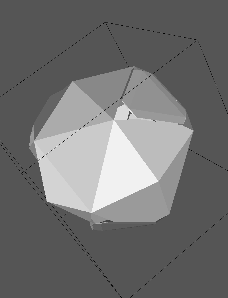
From the cavity.off file one may generate the following plot. Notice how coarse the tesselation is:
Let us know highlight the additional information contained in the output:
a summary of the setup of the PCM calculation is printed out when the Hamiltonian definition is completed:
 ===== Polarizable Continuum Model calculation set-up =====
* Polarizable Continuum Model using PCMSolver external module:
  . Converged potentials and charges at tesserae representative points written on file.
  . Calculate the SS block of the electrostatic potential matrix.
  . Separate potentials and apparent charges in nuclear and electronic.
  . Form One-Index Transformed ASC in a Linear Response calculation.
  . Print potentials at tesserae representative points.


* PCMSolver, an API for the Polarizable Continuum Model electrostatic problem. Version 1.0.0
  Main authors: R. Di Remigio, L. Frediani, K. Mozgawa
   With contributions from:
    R. Bast            (CMake framework)
    U. Ekstroem        (automatic differentiation library)
    J. Juselius        (input parsing library and CMake framework)
  Theory: - J. Tomasi, B. Mennucci and R. Cammi:
           "Quantum Mechanical Continuum Solvation Models", Chem. Rev., 105 (2005) 2999
  PCMSolver is distributed under the terms of the GNU Lesser General Public License.
the PCMSolver module is initialized. The cavity is formed, discretized and the PCM matrix is created. A report is printed out:
~~~~~~~~~~ PCMSolver ~~~~~~~~~~
Using CODATA 2010 set of constants.
Input parsing done API-side
========== Cavity
Cavity type: GePol
Average area = 357.106 AU^2
Probe radius = 2.61727 AU
Number of spheres = 5 [initial = 5; added = 0]
Number of finite elements = 80
========== Solver
Solver Type: IEFPCM, isotropic
PCM matrix hermitivitized
============ Medium
Medium initialized from solvent built-in data.
Solvent name:          Water
Static  permittivity = 78.39
Optical permittivity = 1.776
Solvent radius =       1.385
.... Inside
Green's function type: vacuum
.... Outside
Green's function type: uniform dielectric
Permittivity = 78.39
The parameters chosen in the PCMSolver input are printed out. The number of finite elements generated for the cavity surface are also reported. The final section reports the value for the dielectric constant of the medium.
at each iteration, the time spent in calculating the MEP and ASC is printed out:
* NucMEP evaluation (CPU): 0.00000000s
* NucASC evaluation (CPU): 0.00000000s
* EleMEP evaluation (CPU): 0.00265500s
* EleASC evaluation (CPU): 0.00000000s
Since the .SEPARATE keyword was given, nuclear and electronic MEP and ASC are handled separately.
at each iteration, the MEP and ASC at cavity points are printed out. This is because the printlevel was set to 6 Here it’s just a sample of the printout:
                                                         MEP and ASC at iteration           2
Finite element #          Nuclear MEP                        Nuclear ASC                        Electronic MEP                     Electronic ASC
     1                     3.124762515511                    -0.279550006743                    -3.115288065165                     0.277466656220
     2                     3.124762515511                    -0.279550006743                    -3.115288065165                     0.277466656220
     3                     3.124762515511                    -0.279550006743                    -3.115288065165                     0.277466656220
     4                     3.100728688114                    -0.295176115078                    -3.099377710696                     0.296736937089
the polarization energy components are also reported:
Polarization energy components
   U_ee =   -30.13519885926173 , U_en =    30.18510529332953 , U_ne =    30.18510529332955 , U_nn =   -30.23554041057662
together with a more comprehensive report on the energy at the current iteration:
                            Output from ERGCAL
                            ------------------

Total electronic energy            :   -62.564643386729145
Nuclear potential energy           :    25.365934555796475
Polarization energy                :    -0.000264341589633
Total energy                       :   -37.198973172522301
the polarization energy reported from ERGCAL is the sum of the componets divided by 2.
at the end of each iteration the time spent in forming the PCM Fock matrix contribution is reported:
* PCM Fock matrix contribution (CPU): 0.00269899s
when the calculation is converged, the final energy report lists also the solvation energy, which is the sum of the polarization energy components divided by 2. The total energy already includes this contribution:
                               TOTAL ENERGY
                               ------------

Electronic energy                        :    -62.567437447656800

Other contributions to the total energy
Nuclear repulsion energy                 :     25.365934555796475
Solvation energy                         :     -0.000171652208014

Sum of all contributions to the energy
Total energy                             :    -37.201674544068339
A nonrelativistic Hartree-Fock calculation using two input files
In this tutorial, the input to the PCMSolver module will be provided within the DIRAC input file by adding the *PCMSOLVER section. Read the documentation for this section in the reference manual for further details. Notice that this PCMSolver input is identical to the one given above in the separate file:
**DIRAC
.WAVE FUNCTION
**HAMILTONIAN
.NONREL       ! activates also point nuclei
*PCM
.PRINT
 6
*PCMSOLVER
.CAVTYPE
 GEPOL
.NOSCALING
.AREATS
 100
.SOLVERTYPE
 IEFPCM
.SOLVNT
 WATER
**WAVE FUNCTION
.SCF
*SCF
.PRINT
1
*END OF
The calculation is now run with:
pam --inp=nonrel.inp --mol=CH4.mol
The PCMSolver report now is given by:
~~~~~~~~~~ PCMSolver ~~~~~~~~~~
Using CODATA 2010 set of constants.
Input parsing done host-side
========== Cavity
Cavity type: GePol
Average area = 357.106 AU^2
Probe radius = 2.61727 AU
Number of spheres = 5 [initial = 5; added = 0]
Number of finite elements = 80
========== Solver
Solver Type: IEFPCM, isotropic
PCM matrix hermitivitized
============ Medium
Medium initialized from solvent built-in data.
Solvent name:          Water
Static  permittivity = 78.39
Optical permittivity = 1.776
Solvent radius =       1.385
.... Inside
Green's function type: vacuum
.... Outside
Green's function type: uniform dielectric
Permittivity = 78.39
the only difference being that the module reports that input parsing has been done host-side. Since we didn’t specify the .SEPARATE keyword the total MEP and ASC are reported at tesserae centers for each iteration. The polarization energy components are no longer showed.
A Dirac-Coulomb DFT calculation
In this tutorial we will perform a DFT calculation using the Dirac-Coulomb Hamiltonian and the LDA functional:
**DIRAC
.WAVE FUNCTION
**HAMILTONIAN
.DFT
 LDA
.PCM
*PCM
.PRINT
 6
**WAVE FUNCTION
.SCF
*SCF
.PRINT
 1
*END OF
We use the three files input strategy, as we want to customize both the cavity formation and the solvent selection:
Units = Angstrom
Medium {
     SolverType = CPCM
     ProbeRadius = 1.385
     Solvent = Explicit
     Green<inside> {Type=Vacuum}
     Green<outside> {
                     Type = UniformDielectric
                     Eps = 15.04
     }
}

Cavity {
            Type = GePol
            Area = 100.0
            Mode = Atoms
            Atoms = [1]
            Radii = [1.55]
}
Instead of using the IEFPCM we ask for the CPCM (Conductor-PCM), the solvent is also explicitly specified. The module is currently limited to the handling of homogeneous, uniform, isotropic dielectrics. The cavity is also customized. We use the atomic positions provided in the .mol file, but instead of using the built-in value of 1.70 angstrom for the radius of atom 1 (carbon) we use 1.55 angstrom. The calculation is run as usual and there is nothing more to highlight about the output in this case. Notice that the solvent and solver specification could also be given using the two file input strategy. The specification of custom cavities is only possible with the three file input strategy.
A Dirac-Coulomb, Hartree-Fock, PCM-SCC calculation
As explained in [DiRemigio2015], the calculation of the molecular electrostatic potential integrals:
needed for the PCM can be sped up by neglecting the Small-Small block and replacing the SS block of the potential by a simple Coulombic correction [Visscher1997a]. This approximation is named PCM-SCC and the user can exploit it by specifying the .SKIPSS keyword in the *PCM section of the input:
**DIRAC
.WAVE FUNCTION
**HAMILTONIAN
.PCM
*PCM
.SKIPSS
.PRINT
 6
**WAVE FUNCTION
.SCF
*SCF
.PRINT
 1
*END OF
The PCM-SCC approximation makes sense only when the Dirac-Coulomb Hamiltonian is employed, Notice that by default this integrals are never neglected in a PCM calculation. The user should exercise some care in using this option and test, when feasible, the impact on results of the PCM-SCC approximation.