Computing Electronic Excitations using the Propagator Module POLPRP
Introduction
We want to calculate absorption spectra corresponding to electronic excitations in atoms and molecules. Hereby the absorption energies and the corresponding transition moments are of predominant interest. The POLPRP module allows for the spectra calculation in the valence region of atoms and molecules with an accuracy very simliar to CC-2. The numerical solution of the underlying polarization propagator (POLPRP) is based on the ADC-Method (algebraic diagrammatic construction). This terminology is a bit outdated since the emergence of intermediate state representation technique (ISR) where a correlated many-particle basis is constructed by application of perturbation theory. By this, size-consistency of the method can be achieved. At the same time the obtained eigenvectors which represent a particular excited state carry information about the degree of single-particle character of the excitation and the full configuration information in terms of particle-hole and 2p-2h contributions.
Currently, the strict second-order and the extended second-order ADC schemes are available for the solution of the polarization propagator.
Considerations before submitting a POLPRP job
The excitation space is constructed from all active occupied and virtual orbitals given to MOLTRA. From this a very large number of possible excited configurations emerges also spanning a large energy range. For valence excitations only the lowest excitation energies are relevant implying a Davidson diagonalization scheme as the most suitable one.
The calculation requires a SCF/MOLTRA step for calculation of energies only. If one is interested in configuration information one should also do a Mulliken population analysis. Hereby it is strongly recommended to combine similar orbital types into one group label (via the .LABDEF directive, see there) in order not to be flooded with too verbose information not adding to the physical content. For the transition moments the dipole moment integrals in MO basis are needed. Our first example of the argon atom will cover all these aspects in detail.
The results obtained have to be interpreted properly depending of the type of Hamiltonian used:
- NONREL: You can used contracted basis sets, only the large component basis is used. In the various ireps of the final states you will find the singlet and one or more triplett components. In the absence of SOC tripletts acquire zero transition moments (implying zero oscillator strengths) but the energies are calculated anyhow. For the classification of the individual ireps the same principles as for RELCCSD apply. A combination of linear symmetry and NONREL is not (yet) possible. The highest available symmetry is D2h.
- SPINFREE: Same spin manifolds as for NONREL but you include all scalar relativistic effects up to infinite order. Triplett final states get no osc. strength.
- Four-component (default): The number of available final state ireps is very much reduced and the final states can no longer be classified as pure singlets or pure triplets. Depending on the nuclear charge the former (degenerate) triplet components will now undergo further splitting. One can normally identify the degenerate (SOC-free) parent state without any problems.
- X2Cmmf: The results behave exactly the same way as in the four-component case but you harvest all the advantages of the X2Cmmf method. In the valence space no loss of accuracy with respect to 4C was observed.
Creating POLPRP input (here: excitation spectrum of argon)
Our argon molecular input file contains a basis with enough diffuse functions for a reasonably good result. This way of giving the basis is a bit outdated but was necessary in order to exactly compare to another (nonrelativistic) calculation. Any other basis from the basis set directory can be used as well.
INTGRL
Special Argon basis for production results
D2h symmetry
C   1    3  Z  Y  XA
       18.    1
AR      0.00000000      0.00000000     0.0000000000
LARGE EXPLICIT  3    2    2    2
# s functions
f   9    0
  118022.40
  17683.500
   4027.800
   1145.400
    377.1600
    138.1600
    54.98900
    23.17100
    7.377900
f   9    0
    2.923700
    0.650400
    0.232800
    0.025000
    0.002048
    0.001324
    0.000893
    0.000624
    0.000450
# p functions
f   6    0
    663.0600
    157.0900
    50.23100
    18.63500
    7.446500
    3.095700
f   5    0
    1.106500
    0.415600
    0.145400
    0.050000
    0.020000
# d functions
f   5    0
    1.500000
    0.375000
    0.125000
    0.058700
    0.027600
f   4    0
    0.014204
    0.008017
    0.004927
    0.003175
FINISH
The complete input (here with line numbers) reads as
     1	**DIRAC
     2	.TITLE
     3	Ar exc./X2Cmmf/ADC-2s/D2h/Pop anal./Tr. mom.
     4	.WAVE F
     5	.ANALYZE
     6	**GENERAL
     7	**INTEGRALS
     8	*READIN
     9	.UNCONTRACT
    10	**HAMILTONIAN
    11	.X2Cmmf
    12	**WAVE FUNCTIONS
    13	.SCF
    14	.POLPRP
    15	*SCF
    16	.CLOSED SHELL
    17	 6  12
    18	**ANALYZE
    19	.MULPOP
    20	*MULPOP
    21	.VECPOP
    22	1..oo
    23	1..oo
    24	**MOLTRA
    25	.ACTIVE
    26	 energy -30.0 500.0 0.01
    27	 energy -30.0 500.0 0.01
    28	.PRPTRA
    29	*PRPTRA
    30	.OPERATOR
    31	 XDIPLEN
    32	.OPERATOR
    33	 YDIPLEN
    34	.OPERATOR
    35	 ZDIPLEN
    36	**POLPRP
    37	.DOTRMO
    38	.PRINT
    39	 1
    40	**DAVIDSON
    41	.DVROOTS
    42	 40
    43	.DVMAXSP
    44	 400
    45	.DVMAXIT
    46	 12
    47	.DVCONV
    48	 1.0E-06
    49	*END OF
The UNCONTRACT directive (9) is unnecessary here since we plug in an uncontracted set. In a relativistic calculation with SOC contracted basis sets need to be decontracted, however. To activate POLPRP we specify it in the wave function section (14). Furthermore we need Mulliken analysis (18) also for the virtuals (21,22,23). In the MOLTRA section we see that all occupied orbitals and nearly all virtuals are included in the active space (26,27). As mentioned above, for the calculation of transition moments we need the dipole moment integrals in MO basis which is triggered in lines 28-35 of the MOLTRA section. In the POLPRP section we indicate that we want to compute TMs (.DOTRMO) and all ireps where a possible final state can occur are calculated because the .STATE keyword was omitted. Then the program determines all these symmetries by itself. The Print directive in line 38/39 is required to generate the orbital list of active occupied and virtual spinors. You need this orbital list if the postprocessing tools are to be used. The DAVIDSON section controls the iterative diagonalizer that is always called in conjunction with POLPRP. The additionally available LANCZOS diagonalizer used in the one- and two-particle propagators is not applied here and can not be called. The keywords are described in the manual and choosing reasonable values needs a little bit of experience with iterative diagonalizers. The DVMAXSP determines the maximum size of the Hamilton operator projection (the Krylov space) and strongly influences memory demands of the routine.
Working with the output files
Besides the usual Dirac .out file where a lot of technical information of the POLPRP calculation is printed some essential result files are produced that can be used for further analysis and postprocessing. These are the file ADCEVECS.XX, ADCSTATE.XX and ADCTRMOM (the latter only if TMs were activated). XX here stands for the corresponding irep number that can be 01..32 at most (linear case).
The ADCEVECS.XX files contain the eigenvectors of the large ADC matrix in binary form and can be used for restarts of the module. If copied to the scratch directory, the module reads them in and starts from these already converged eigenvectors.
The ADCSTATE.XX file contains human-readable information about the eigenstates of irep XX where the most important configurations appear first:
Excited state:    1
 -----------------
Exc. energy:  0.461708 au  12.563724 eV  PS:  0.960574 Err:  0.000033 Sym:   1
Norm^2 of double exc. contr:       0.039426

128 ( 3, 1Eu)  <----   9 ( 3, 1Eu)   0 ( 0,    )  <----   0 ( 0,    )        0.355139          0.126124
152 ( 4, 2Eu)  <----  15 ( 4, 2Eu)   0 ( 0,    )  <----   0 ( 0,    )       -0.355139          0.126124
151 ( 4, 2Eu)  <----  16 ( 4, 2Eu)   0 ( 0,    )  <----   0 ( 0,    )        0.348944          0.121762
127 ( 3, 1Eu)  <----  10 ( 3, 1Eu)   0 ( 0,    )  <----   0 ( 0,    )       -0.348944          0.121762
129 ( 3, 1Eu)  <----   8 ( 3, 1Eu)   0 ( 0,    )  <----   0 ( 0,    )       -0.226284          0.051205
153 ( 4, 2Eu)  <----  14 ( 4, 2Eu)   0 ( 0,    )  <----   0 ( 0,    )        0.226284          0.051205
154 ( 4, 2Eu)  <----  16 ( 4, 2Eu)   0 ( 0,    )  <----   0 ( 0,    )        0.184017          0.033862
130 ( 3, 1Eu)  <----  10 ( 3, 1Eu)   0 ( 0,    )  <----   0 ( 0,    )       -0.184017          0.033862
155 ( 4, 2Eu)  <----  15 ( 4, 2Eu)   0 ( 0,    )  <----   0 ( 0,    )       -0.156695          0.024553
131 ( 3, 1Eu)  <----   9 ( 3, 1Eu)   0 ( 0,    )  <----   0 ( 0,    )        0.156695          0.024553
128 ( 3, 1Eu)  <----  10 ( 3, 1Eu)   0 ( 0,    )  <----   0 ( 0,    )        0.153918          0.023691
152 ( 4, 2Eu)  <----  16 ( 4, 2Eu)   0 ( 0,    )  <----   0 ( 0,    )       -0.153918          0.023691
127 ( 3, 1Eu)  <----   9 ( 3, 1Eu)   0 ( 0,    )  <----   0 ( 0,    )        0.136675          0.018680
151 ( 4, 2Eu)  <----  15 ( 4, 2Eu)   0 ( 0,    )  <----   0 ( 0,    )       -0.136675          0.018680
Hereby the excitation energy of the first state in symmetry (irep) 1 is given in au and eV and PS stands for pole strength which is a bit misleading in this context but describes the percentage of single-excitation character of this particular final state (96.06%). The next entry is the residual error stemming from the Davidson diagonalizer. Obviously, the next line tells us that we have 3.94 % double excitation character.
The following rows now reveal the leading configurations this state is composed of. First let us focus on the two rightmost columns with expansion coefficients (ISR basis!) and their squares. It is observed that these coefficients are pairwise identical apart from a sign reflecting the fact of Kramers pairing. All spinors occur twice in the corresponding Kramers ireps and possess identical orbital energies. Therefore the expansion distributes equally over both possible one-particle configurations. The first number gives the absolute spinor number with respect to the active orbital list and the number in parenthesis is the relative spinor number within the given irep. The corresponding first line tells us that our first expansion term consists of a single-particle excitation from occupied spinor 9 into virtual spinor 128 with a coefficient of 0.355139 etc. The other zeros indicate the single-particle character of this excitation and get nonzero for a 2h–>2p type. In the framework of ISR and perturbation theory one can approximately think of expansion determinants that are described here. Strictly speaking, these are correlated singly excited configurations. By analyzing all ADCSTATE.XX files you can generate a complete spectrum but without proper utilities (see below) this can become a bit tedious. The utilities can be obtained from the author of this module.
Let’s now turn to the ADCTRMOM file that is generated when we asked for transition moments. Actually, there is only one file collecting the information of all symmetries:
*********************************************
**  Final State Symmetry:            1
*********************************************


State   1 symm   1 exc. energy    0.461708 (au)    12.563724 (eV)   PS    0.960574   @E
Order               TM(x)_r        TM(x)_i          TM(y)_r        TM(y)_i          TM(z)_r        TM(z)_i
   0th            0.000000000    0.000000000 |     0.000000000    0.000000000 |     0.000000000    0.000000000
   1st            0.000000000    0.000000000 |     0.000000000    0.000000000 |     0.000000000    0.000000000
   2ndA           0.000000000    0.000000000 |     0.000000000    0.000000000 |     0.000000000    0.000000000
   2ndB           0.000000000    0.000000000 |     0.000000000    0.000000000 |     0.000000000    0.000000000
   2ndC           0.000000000    0.000000000 |     0.000000000    0.000000000 |     0.000000000    0.000000000
   2nd 2,1        0.000000000    0.000000000 |     0.000000000    0.000000000 |     0.000000000    0.000000000
   2nd 2,2        0.000000000    0.000000000 |     0.000000000    0.000000000 |     0.000000000    0.000000000
   2nd 2,3        0.000000000    0.000000000 |     0.000000000    0.000000000 |     0.000000000    0.000000000
   2nd 2,4        0.000000000    0.000000000 |     0.000000000    0.000000000 |     0.000000000    0.000000000
   2nd 2,5        0.000000000    0.000000000 |     0.000000000    0.000000000 |     0.000000000    0.000000000
   2nd 2,6        0.000000000    0.000000000 |     0.000000000    0.000000000 |     0.000000000    0.000000000
   2nd 2,7        0.000000000    0.000000000 |     0.000000000    0.000000000 |     0.000000000    0.000000000
   2nd 2,8        0.000000000    0.000000000 |     0.000000000    0.000000000 |     0.000000000    0.000000000
   2nd 2,9        0.000000000    0.000000000 |     0.000000000    0.000000000 |     0.000000000    0.000000000
   2nd 2,10       0.000000000    0.000000000 |     0.000000000    0.000000000 |     0.000000000    0.000000000
   2nd 2p2h A     0.000000000    0.000000000 |     0.000000000    0.000000000 |     0.000000000    0.000000000
   2nd 2p2h B     0.000000000    0.000000000 |     0.000000000    0.000000000 |     0.000000000    0.000000000
------------------------------------------------------------------------------------------------------------
   total          0.000000000    0.000000000 |     0.000000000    0.000000000 |     0.000000000    0.000000000
   Osc. strength:     -->>        0.00000000  a.u.      @O
------------------------------------------------------------------------------------------------------------
The first line is more or less reproducing the entries in ADCSTATE.XX. Next comes a detailed list of individual x,y,z contributions to the transitions moments for each perturbational order and type of contraction. This is a speciality of the ADC method and allows for detailed insights into individual contributions to the TM. TMs can be complex, so both real and imaginary parts are given. The oscillator strength is calculated according to the usual formula using the sum of squares of Tx, Ty and Tz. For easy grepping of energies and oscillator strengths in production the markers “@E” and “@O” were introduced.
In order to collect all the peaks representing an excited final state together with their oscillator strengths from the ADCTRMOM file you can do the following:
grep '@E' ADCTRMOM|cut -c1-84 > ex; grep '@O' ADCTRMOM|cut -c30-52 > os; paste ex os > stickspectrum
These lines generate the text file ‘stickspectrum’ with all relevant information of the excited states. Hereby all states within a specific symmetry are listed together. This file can already be used for the generation of a simple gnuplot graph where we draw the peak heights/vs energies.:
plot [:][0:1.0] "stickspectrum" u 9:12 w i lw 2
Keep in mind that this command plots all peaks irrespective of their experimental observability which is described by the oscillator strength! (shaping up the graph is not discussed here)
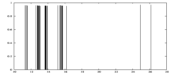
We see that all peaks exhibit nearly the same height around 0.95. This points to prevailing single excitation character but does not relate to experimental observability. Certainly, the obtained result is not ready for comparison with experiment. In order to arrive at physically meaningful spectra we refer you to the second chapter of the Spectroscopy II tutorial where we compute the excitation spectrum of the transition metal complex H2Os(CO)4 in full scope and with additional utilites necessary to generate it. In the following section we address some aids to interpret the Dirac .out file.
Comments on the POLPRP output (in order of appearance)
- The property handler is called when you ask for transition moments. It prepares the dipole moment integrals represented in MO basis.
- Generating (real/complex) Dav. start vectors (all symm.): The particle/hole matrix that is calculated for all possible symmetries at once is diagonalized and corresponding eigenvectors are written out that serve as start vectors for the Davidson iteration (file DAVSTART.XX). If you obtain a warning that Hermiticity is violated in the p/h blocks something serious wnet wrong. Check the list of active orbitals then.
- Constructing real satellite part. In this section the coupling and satellite blocks of the ADC matrix are constructed and written out to disk (file: PP_ELE). In parallel runs this matrix is distributed over the compute nodes (files: PP_ELE.XX). Some dimensions and block sizes are reported as well.
- The Davidson algorithm output reports about dimensions, start vectors, orthogonality (important!) and user input.
During the diagonalization you will be prompted the progress as:
 root    dim       exc.energy       error     status  time/root (s)
----------------------------------------------------------------------
Time for constructing Krylov projection     19.97
Time for constructing residual vectors      6.89

   1      40       0.5342178       0.5190262 o    XT                0.16
   2      41       0.5453888       0.5187599 o    XT                0.17
   3      42       0.5453888       0.5187599 o    XT                0.17
   4      43       0.5453888       0.5187599 o    XT                0.17
The ‘XT’ abbreviation hereby indicates a successful extension of the Krylov space by using the computed preconditioner. The small ‘o’ denotes a nonconverged root whereas a ‘*’ points to a converged one. Converged roots are no longer touched in the algorithm increasing the efficiency. It can also happen that the preconditioner cannot determine a vector possessing enough orthogonality to the already converged space. In this case a warning is issued and you should carefully examine the quality of your calculations at the end of the run. A macroiteration denotes a cycle of one complete Krylov space construction followed by collapsing the space (see publication for more details).
The verbose output in case of transition moment calculation can be more or less ignored because it is summarized in the ADCTRMOM file. In the near future we will considerably shrink the output of POLPRP but for the moment it provides a high level of detail useful for the analysis of difficult cases.
The sequence just described is now repeated for all ireps separately. It is a big advantage of the ADC/ISR method that the representation matrices exhibit full block structure. So each symmetry (irep) can be treated independently and the user can select the desired ireps by the .STATE directive (see manual).