Calculation of electric properties in solution: dipole moments and polarizabilities
The current implementation of the PCM in DIRAC allows for the calculation of electric properties up to second order. This means that electric dipole moments and electric dipole polarizabilities are available.
The analytical results can also be checked against a finite-field approach. The Hamiltonian defined In the input the Hamiltonian definition is augmented by an explicit electric field. Repeating the calculation with different coupling strengths and electric field directions, will enable the use of a stencil formula for the finite-difference calcultion of energy derivatives, for example using a Five-point stencil:
Electric dipole moments
We recall that the component \(I\) of the electric dipole moment is defined as the first derivative, at zero perturbation strength, of the energy with respect to the component \(I\) of an applied external electric field \(\mathbf{F}\).
Thanks to the Hellmann-Feynman theorem, this reduces to the calculation of the expectation value of the component \(I\) of the electric dipole moment operator:
Calculation of dipole moments with PCM is quite straightforward. We just need to add the PCM section to a dipole moment calculation input file:
**DIRAC
.WAVE FUNCTION
.PROPERTIES
**HAMILTONIAN
.PCM
**WAVE FUNCTION
.SCF
**PROPERTIES
.DIPOLE
*END OF
and of course use the appropriate PCMSolver input file:
Units = Angstrom
Medium {
     SolverType = CPCM
     Solvent = Cyclohexane
}

Cavity {
            Type = GePol
            Area = 10.0
            Mode = Explicit
            Spheres = [0.0, 0.0, 0.0, 20.0]
}
This PCMSolver input file requires the CPCM model with cyclohexane as solvent. The solute is enclosed in a cavity made from a single sphere, centered at the origin and with a 20 angstrom radius. Consider the following .mol file for water as an example:
INTGRL
Water

C   2    0
        8.    1
O      .0000000000        0.0000000000        -.2249058930
LARGE BASIS cc-pVDZ
        1.    2
H     1.4523499293         .0000000000         .8996235720
H     -1.4523499293         .0000000000         .8996235720
LARGE BASIS cc-pVDZ
FINISH
The output for the dipole moment calculation looks just like usual:
    **************************************************************************
    *************************** Expectation values ***************************
    **************************************************************************

                                                   s0 t0
----------------------------------------------------------------------------
    Dipole length: X :     0.63076018E-12 a.u.      F   F
    Dipole length: Y :    -0.20258107E-15 a.u.      F   F
    Dipole length: Z :     0.813178997624 a.u.      F   F
----------------------------------------------------------------------------
    s0 = T : Expectation value zero by point group symmetry.
    t0 = T : Expectation value zero by time reversal symmetry.
----------------------------------------------------------------------------
* Dipole moment:

          Electronic               Nuclear                  Total
          contribution             contribution             contribution
----------------------------------------------------------------------------
x         0.00000000 Debye         0.00000000 Debye         0.00000000 Debye
y        -0.00000000 Debye         0.00000000 Debye        -0.00000000 Debye
z         2.06691398 Debye         0.00000000 Debye         2.06691398 Debye
----------------------------------------------------------------------------
x         0.00000000 a.u.          0.00000000 a.u.          0.00000000 a.u.
y        -0.00000000 a.u.          0.00000000 a.u.         -0.00000000 a.u.
z         0.81317900 a.u.          0.00000000 a.u.          0.81317900 a.u.
----------------------------------------------------------------------------

 1 a.u =   2.54177000 Debye
Electric dipole moment polarizabilities
We recall that the electric dipole polarizability is a second order property as is defined as the second derivative, at zero field strength, of the energy:
In a response theory framework, the polarizability tensor elements can be identified from the linear response function, see [Saue2002a]:
The polarizability is a rank-2 tensor and has six unique components. We can extract two invariant quantities from the tensor: the isotropic and anisotropic polarizability:
Again, we just need to add the PCM section to an electric dipole polarizability calculation input file:
**DIRAC
.PROPERTIES
**HAMILTONIAN
.PCM
**WAVE FUNCTION
.SCF
**PROPERTIES
.POLARIZABILITY
*END OF
the same .mol file as above for water is used in this example. The following PCMSolver input file is used:
Units = Angstrom
Medium {
                Solvent = Water
}

Cavity {
                Type = GePol
                Area = 10.0
                Mode = Implicit
}
The output for the dipole moment calculation looks just like usual:
                    +--------------------------------+
                    ! Electric dipole polarizability !
                    +--------------------------------+


@   Elements of the electric dipole polarizability tensor

@   xx            7.76376447 a.u.   (converged)
@   yy            3.21397401 a.u.   (converged)
@   zz            5.57773363 a.u.   (converged)

@   average       5.51849070 a.u.
@   anisotropy    3.941      a.u.

@   xx            1.15047118 angstrom**3
@   yy            0.47626180 angstrom**3
@   zz            0.82653484 angstrom**3

@   average       0.81775594 angstrom**3
@   anisotropy    0.584      angstrom**3
Influence of the relative permittivity on electric properties
It is interesting to analyze the effect of varying the relative permittivity of the solvent on the calculation of electric properties. We will use the two input files strategy and exploit the string substitution mechanism of the pam scripti. Consider the pcm-prop.inp input file:
**DIRAC
.WAVE FUNCTION
.PROPERTIES
.PCM
*PCM
*PCMSOLVER
.CAVTYPE
 GEPOL
.NOSCALING
.AREATS
 10
.SOLVERTYPE
 IEFPCM
.SOLVNT
 solvent
**WAVE FUNCTION
.SCF
**PROPERTIES
.DIPOLE
.POLARIZABILITY
*END OF
Notice that instead of specifying a solvent name we put a placeholder string. This can be exploited to run calculations selecting a different solvent:
pam --inp=pcm-prop.inp --replace solvent=CYCLOHEXANE --mol=H2O.mol
or run this in a loop:
# Declare array of solvents. Solvents are ordered by increasing relative permittivity
declare -a solv_array=("N-HEPTANE" "CYCLOHEXANE" "CARBON TETRACHLORIDE" "BENZENE" "TOLUENE" "CHLOROFORM" "CHLOROBENZENE" "ANILINE" "TETRAHYDROFURANE" "METHYLENECHLORIDE" "1,2-DICHLOROETHANE" "ACETONE" "ETHANOL" "METHANOL" "ACETONITRILE" "NITROMETHANE" "DIMETHYLSULFOXIDE" "WATER")

# Now loop over the array elements and substitute them to the string solvent in pcm-prop.inp
for solv in "${solv_array[@]}"
do
    echo "$solv"
    pam --inp=pcm-prop.inp --replace solvent=$solv --mol=H2O.mol
done
This will produce a different output file for every different solvent in the array. One can collect the results for dipole moments and isotropic polarizabilities and plot them against the relative permittivities. This was done in [DiRemigio2015] for the \(\mathrm{H}_2\mathrm{Po}\) molecule:
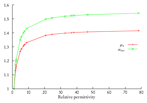
where it was also found that the difference between the values of the observables in solution and in vacuo can be fitted to a linear rational function:
An analogous relation was found to be valid also for the dipole moment. Notice that the \(a, b\) coefficients are system-dependent.